This page will describe more advanced techniques of looking up data, especially looking up data by two key values, instead of one. We'll begin with the following example.
Double Lookups
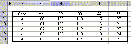
You can't use the VLOOKUP function to do a double lookup -- that is, a lookup based on both the row headers (column F) and the column headers (row 8). Suppose we want to return the value with a row header value of c and a column header value of 44. We can't use either VLOOKUP or HLOOKUP in this situation, because each of these functions can search only in one direction. Instead we use the MATCH and OFFSET functions.
=OFFSET($F$8,MATCH(F16,$F$9:$F$13,0),MATCH(G16,$G$8:$K$8,0))
In this example, cell F16 contains the desired row header (c) and cell G16 contains the desired column header (44). This function uses OFFSET to return a cell reference a specified number of row and columns from a particular cell -- in the example this "base" cell is F8. The two MATCH functions return the row and column offsets of the data. Here, the formula MATCH(F16,$F$9:$F$13,0) returns 3, because the value c is the third value in the range $F$9:$F$13. Similarly, the function MATCH(G16,$G$8:$K$8,0) returns 4, because 44 is the fourth value in the range $G$8:$K$8 . When these values are passed into OFFSET, it returns the cell that is 3 rows and 4 columns from F8.
Left Lookups
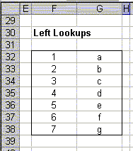
=OFFSET(G32,MATCH(I32,$G$32:$G$38,0)-1,-1,1,1)
The MATCH function tells us where in the list $G$32:$G$38 the value of I32 is, and then the OFFSET function goes to the left ( -1) to retrieve the value.
Arbitrary Lookups
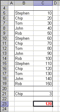
The following array formula will return the value from column C corresponding to a specified value in column B. That value is named in cell B21, and the occurrence is specified in cell C21.
=INDEX(B5:C19,SMALL(IF(B5:B19=B21,ROW(B5:B19)-ROW(B5)+1,ROW(B19)+1),C21),2)
In the example on the left, the data to search is in
the range B5:C19.
The value in column B to search for, Chip, is specified in cell
B21,
and the occurrence of that value, 3, is specified in cell
C21.
The result of this formula is 120, because 120 corresponds to the 3rd
occurrence of Chip in column B.
If you want to lookup the last occurrence of a value in the list, you can
use the following array formula.
=INDEX(B5:C19,SMALL(IF(B5:B19=B21,ROW(B5:B19)-ROW(B5)+1,ROW(B19)+1),COUNTIF(B5:B19,B21)),2)
This is the same formula as above, but the reference to
C21 has been replaced by the function
COUNTIF(B5:B19,B21),
which will count the number of values equal to
B21
in the range B5:B19.
Remember, these are array formulas, so you must press
Ctrl+Shift+Enter rather than just Enter
when you first enter the formula and whenever you edit it later. If you do
this correctly, Excel will display the formula enclosed in curly braces
{ }.
Closest Match Lookups
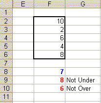
The following formula will return the value from cells
F2:F6
that is closest to, but not less than, the value in
F8.
For example, in the list shown to the left, the formula will return 8,
because 8 is closest to the value 7, in
F8,
without exceeding it.
=INDEX(F2:F6,MATCH(MIN(IF(F2:F6-F8>=0,
F2:F6,FALSE)),IF(F2:F6-F8>=0,F2:F6,FALSE),0))
We can write a similar formula to return the value that is closest to, but
not greater than, a given value. Referring to the list at the left,
the following formula will return 6, because 6 is closest to, but not
greater than, 7.
=INDEX(F2:F6,MATCH(MAX(IF(F2:F6-F8<=0,
F2:F6,FALSE)),IF(F2:F6-F8<=0,F2:F6,FALSE),0))
Remember, these are array formulas, so you must press
Ctrl+Shift+Enter rather than just Enter
when you first enter the formula and whenever you edit it later. If you do
this correctly, Excel will display the formula enclosed in curly braces
{ }.
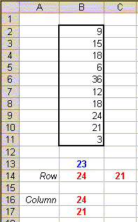
=INDEX(B2:B11,MATCH(SMALL(ABS(B2:B11-B13),
{1,2}),ABS(B2:B11-B13),0))
Since this formula returns two values, you must enter it into an array of two cells. First select the two cells which you want to contain the results, and then type the formula. Be sure to press Ctrl+Shift+Enter rather than just Enter when you enter the formula. Because this formula is in an array of cells, you won't be able to edit each cell independently. To change the formula, you must select both cells, edit the formula, and then press Ctrl+Shift+Enter when you're done.
As written, the formula returns its results in to two cells in the same row, say B14:C14. If you want to return the values to two cells in the same column, say B16:B17, use the formula below.
=INDEX(B2:B11,MATCH(SMALL(ABS(B2:B11-B13),
{1;2}),ABS(B2:B11-B13),0))
This is the same formula as the previous formula, but the row array {1,2} is changed to a column array {1;2}. Notice that these are enclosed in curly braces {}, not parentheses.
You can download an example workbook with these
formulas here.