 Tables And Lookups
This page describes a number of formulas to return data from tables and formulas to look up data in tables.

Almost every worksheet contains at least one table of data, typically a set of rows and columns. Very frequently, you will need to
return a row or column of values from the table the row or column position in the table, or you may need to return a value
from the table based upon a match of values in the row headers and column headers. For example, you may need to return the 5th row
of a table, or you may need to return the row where the ID number is 1234.
The simplest types of lookups are performed with the
VLOOKUP or HLOOKUP functions. The functions are well documented in the Help
file and are not discussed in detail on this page. It is assumed that you are familiar with VLOOKUP and
HLOOKUP. For more complicated lookups in tables, we will use formulas based on the
OFFSET, MATCH, and INDEX functions. While the Help
file describes these functions individually, it does not describe how these functions can be combined to create more powerful and
flexible lookup formulas. That is the goal of this page. At the core of most of the formulas on this page is the OFFSET
function. You should be familiar with this function before proceeding with this page.
Most of the formulas on this page are array formulas. Array formulas are described in detail on the
Array Formulas page on this web site. You should be at ease with array formulas in order to
modify the lookup formulas presented on this page. With few exceptions, the formulas on this page use only a single range reference,
a Defined Name that refers to the data table against which the lookup is performed. Using a single reference may make the formulas
longer, but it also makes them considerably more flexible. To use the formulas on your own worksheets, you need only modify a
single name. This convenience makes up for, in my opinion, the longer formula length. Of course, if you are not using a defined
name, simply replace the name in the formula with the appropriate range reference.
If the formulas on this page do not return the expected result when you use them on your own worksheets, the first thing to check is
to ensure that the formula is entered as an array formula. If you are unsure whether a formula needs to be array entered, go ahead
and enter it as an array formula; that is completely safe.
ENTERING AN ARRAY FORMULA: When you enter a formula as an array formula, you must press
CTRL SHIFT ENTER rather than just ENTER when you first enter the formula and whenever you edit
it later. If you do this properly, Excel will display the formula in the formula bar enclosed in curly braces,
{ }. You do not type in the curly braces, { }; Excel will display them
automatically.
In the interest of brevity and clarity, the formulas on this page do not have any error checking and handling. For example, there
is nothing to prevent you from attempting to return the 6th row of a table that has only 4 rows. If a parameter in a function
call is invalid, you will most likely get a #N/A error. You may want to add some error checks when
you use these formulas in your own worksheets.
As is the case with many types of formulas in Excel, there are several different ways to accomplish the same thing. Many of the formulas
on this page could be written with a combination of the INDEX and MATCH functions
instead of the OFFSET function. OFFSET is neither better nor worse than
INDEX/MATCH. For consistency, I have chosen to use OFFSET for nearly
all the tasks at hand. Other sources may use other methods. I encourage you to learn a variety of ways to accompish a task.
You can download an example workbook containing all of the formula on this page.

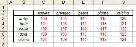
The example formulas in the first section of this page, those formulas for returning rows and columns of a table, use the
following data table.

This table contains two named ranges that are used in the formulas. The name Table refers to the entire
table, cells B2:G7, which includes the row labels and column labels. The name
InnerTable refers only the the actual data, cells C3:G7, which does not include the row labels
and the column labels. For illustration, the values of the row labels (abby, beth, etc.) and the column labels
(apples, oranges, etc) are in alphabetical order. This is for illustration only. The formulas do not require that
the values be in any particular order.

You can use an array formula to return a single row or column from a table. The formulas in this section need to be array entered
(press CTRL SHIFT ENTER rather than just ENTER) into a number of cells equal to
the size of the row or column of the table. The example table contains 6 columns (including the row header); thus, you would select a range
that is 6 columns wide and 1 row tall, enter the formula and press CTRL SHIFT ENTER.
The first formulas return a single row, based on position, from Table or InnerTable.
=OFFSET(Table,E13-1,0,1,COLUMNS(Table))
In this formula, cell E13 contains the row to return. The row is 1-based (the title row is 1, the first row
of data is 2, etc). The OFFSET function uses 0-based rows and columns, so we subtract 1 from the row
number before passing it into the OFFSET function. If cell E13 contains
the number 5, the formula returns the following values:

The following formula returns a row from the InnerTable range. It return only the data values, not the
row header.
=OFFSET(InnerTable,E18-1,0,1,COLUMNS(InnerTable))
In this formula, cell E18 contains the 1-based row of InnerTable to return.
Thus, if cell E18 contains 5, the formula returns the following values.

By changing the values that are passed to the OFFSET function, we can return a column from either the
Table or InnerTable range, either by using a column offset or the value of
a column label. The following formula will return a column from the Table range.
=OFFSET(Table,0,E22-1,ROWS(Table),1)
If cell E22 contains the value 3, the third column of Table is returned, as
shown below:

Since this formula returns a column of data from Table, it should be array entered into to a range that is
one column wide and has the same number of rows and the Table range.
You can also return a column from Table that corresponds to a matching column label. The following formula
will return the column from Table whose column label is equal to the value in cell E39.
=OFFSET(Table,0,MATCH(E39,OFFSET(Table,0,0,1,COLUMNS(Table)),0)-1,ROWS(Table),1)
If cell E39 contains the value plums, the following values are returned.


Because the formulas described above return arrays of values, either a row or column of the InnerTable,
you can use those formulas with functions that accept arrays. Indeed, you can use the row and column functions in any function or
formula where you would normally provide a range of cells, such as in the SUM,
MIN, MAX, or AVERAGE functions, among others.
For example, the following formula will return the SUM of the row whose row label is equal to the value in
cell E48.
=SUM(OFFSET(InnerTable,MATCH(E48,OFFSET(Table,0,0,ROWS(Table),1),0)-2,0,1,COLUMNS(InnerTable)))
If cell E48 contains the value callie, this formula will return the value 560. You can get the
maximum or minimum of the row by changing SUM to MAX or
MIN. These formula do not need to be entered as array formulas, although it is harmless to do so.
A very similar formula can be used to return the sum, minimum, or maximum of a column in the table. The following formula will return
the sum of the values in the column of Table where the column label is equal to the value in cell
E52.
=SUM(OFFSET(InnerTable,0,MATCH(E52,OFFSET(Table,0,0,1,COLUMNS(Table)),0)-2,ROWS(InnerTable),1))
If cell E52 contains oranges, the formula will return 535. As before, you can change
SUM to MIN or MAX to return the minimum or
maximum of the column. Again, these formulas need not be array entered.

You can use a formula to return the last cell in a row or column, where the row or column is select either by its position in the
table or by a match of a value with the row or column label.
The following formula will return the last (right-most) value in a row of Table, where cell
E56 contains the 1-based row position:
=OFFSET(Table,E56-1,COLUMNS(Table)-1,1,1)
If E56 contains 4, the result is 122, the last value in the 4th column of Table
(including the column labels). You also select the row to use by matching a row label. If cell E59 contains
the value callie, the following formula will return 122, the right-most value in the row whose row label is callie.
=OFFSET(Table,MATCH(E59,OFFSET(Table,0,0,ROWS(Table),1),0)-1,COLUMNS(Table)-1,1,1)
The following formulas will return the last (bottom-most) value of a column, selected by either its position in Table
(cell E62) or by a match of a column label (in cell E65).
=OFFSET(Table,E62-1,COLUMNS(Table)-1,1,1)
=OFFSET(Table,ROWS(Table)-1,MATCH(E65,OFFSET(Table,0,0,1,COLUMNS(Table)),0)-1)

A double lookup is a formula that returns a value from a table based on a match of values in both the rows and columns. Refering to the
example data shown above, you may want to return the value corresponding to the dora row and the plums column. If cell
E74 contains the value to match on the rows (e.g., dora) and cell E75
contains the value to match on the columns (e.g., plums), the following formula will return the appropriate value from the
Table range:
=OFFSET(Table,MATCH(E74,OFFSET(Table,0,0,ROWS(Table),1),0)-1,
MATCH(E75,OFFSET(Table,0,0,1,COLUMNS(Table)),0)-1)

While the VLOOKUP function is very useful, it has a significant limitation. That is that you can only
return a value to the right of the lookup column. For example, you can look in column B for a value and then return the corresponding
value from column D. However, the reverse is not true. You cannot look up a value in column D and return the corresponding value
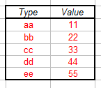
from column B. This is where a Left Lookup formula is useful. For example, suppose you have the following table, and a defined name
of LLTable that refers to the actual data (colored in red).

The following formula will look for a value in the Value column and return the corresponding value in the Type column.
=OFFSET(LLTable,MATCH(F67,OFFSET(LLTable,0,1,ROWS(LLTable),1),0)-1,0,1,1)
In this formula, cell F67 contains the value to be searched for in the Value column. Thus, if
F67 contains 44, the formula will return dd.

The HLOOKUP function is the "transpose" of the VLOOKUP function. As
VLOOKUP scans down a column for a match and then moves to the right to return a value,
HLOOKUP scans across a row for a match and then moves down to return a value. HLOOKUP cannot move
upwards to return a value. For example, you can search row 5 to find a match and then return the corresponding value from row 8, but
the reverse is not possible. You cannot scan row 8 and return a value from row 5. Just as the Left Lookup formula overcame the
limitation of VLOOKUP, an Upper Lookup formula can overcome the limitation of HLOOKUP.
Consider the following table:

In this table, the range displayed in red has the name ULTable. The followng
formula will allow you to look in the Value row for a value equal to cell J82 and return the corresponding
value from the Type row.
=OFFSET(ULTable,0, MATCH(J82, OFFSET(ULTable,ROWS(ULTable)-1,0,1,COLUMNS(ULTable)),0)-1,1,1)
For example, if J82 contains 33, the formula will return cc.

Another limitation of the VLOOKUP function is that if there are duplicate matches in the lookup column,
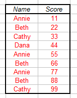
the first occurrence of the matching value is used. For example, consider the following table of data:

With a simple VLOOKUP function for the value Beth, the value 22 will be returned, since 22 corresponds
to the first occurrence of the value Beth. It may be necessary, however, to return the value corresponding to the second or
third occurrence of Beth. If the table of values (colored in red, excluding the
Name and Score column labels) is named ALTable, the following formula will
return the value form the Score column corresponding the the Nth occurrence of the value in cell F90,
where the number N is in cell F91. For example, if F90 contains the value
Beth and cell F91 contains the value 3 (indicating to find the 3rd occurrence of Beth), the
formula will return the value 88.
=INDEX(ALTable,SMALL(IF(OFFSET(ALTable,0,0,ROWS(ALTable),1)=F90,
ROW(OFFSET(ALTable,0,0,ROWS(ALTable),1))-ROW(OFFSET(ALTable,0,0,1,1))+1,
ROW(OFFSET(ALTable,ROWS(ALTable)-1,0,1,1))+1),F91),2)
A special case of the arbitrary lookup formula above is to return the value corresponding to the last occurrence in the list. For
example, if cell F94 contains the value Beth, the following formula will return the value
88, which corresponds to the last occurrence of the value Beth.
=INDEX(ALTable,SMALL(IF(OFFSET(ALTable,0,0,ROWS(ALTable),1)=F94,
ROW(OFFSET(ALTable,0,0,ROWS(ALTable),1))-ROW( OFFSET(ALTable,0,0,1,1) )+1,
ROW(OFFSET(ALTable,ROWS(ALTable)-1,0,1,1))+1),COUNTIF(OFFSET(ALTable,0,0,ROWS(ALTable),1),F94)),2)

The MATCH function is an important tool when working with lists of data. If you are searching for an
exact match in a range of cells, the values may be in any order. However, if you are attempting to find a closest match, the values
must be in sorted order. Using the INDEX and MATCH functions, you can
write a formula that will return the number in a list that is closest to a specified value. We will look at three related
Closest Match formula. These three formulas are based on the example data shown below. All three formulas are
array formulas, so you must enter them with CTRL SHIFT ENTER, not
just ENTER. This list of values has the defined name of CMTable.

The following array formula will return the smallest number in the list CMTable that greater than or
equal to the value in cell E105.
=INDEX(CMTable,MATCH(MIN(IF(CMTable-E105>=0,CMTable,FALSE)),IF(CMTable-E105>=0,CMTable,FALSE),0))
Thus is E105 has the value 5, the formula will return 5.1, which is the smallest number in the list
that is greater than or equal to 5.
The second Closest Match formula will return the largest number in a list that is less than or equal to a specified number. In
the following formula, cell E108 contains the test value.
=INDEX(CMTable,MATCH(MAX(IF(CMTable-E108<=0,CMTable,FALSE)),IF(CMTable-E108<=0,CMTable,FALSE),0))
Thus, if cell E108 has the value 8, the formula will return 7.4, which is the largest number in the
range that is less than or equal to 8.
The third and final Closest Match formula will return the value in a list that is closest to a specified value. The returned value
might be less than the test value or it might be greater than the test value.
=INDEX(CMTable,MATCH(MIN(ABS(CMTable-E111)),ABS(CMTable-E111),0),1)
Thus, if cell E111 contains the value 5, the formula will return 5.1, since 5.1 is closer to 5 than
any other value in the list.
You can download an example workbook containing all of the formula on this page.
This page last updated: 12-April-2009