Array formulas are a powerful tool in Excel. An array formula is a formula that
works with an array, or series, of data values rather than a
single data value. There are two flavors of array formulas: first, there
are those formulas that work with an array or series of data and aggregate it,
typically using SUM, AVERAGE,
or COUNT, to return a single value to a single
cell. In this type of array formula, the result, while calculated from arrays,
is a single value. We will examine this type of array formula first. The second
flavor of array formulas is a formula that returns a result in to two or more
cells. These types of array formulas return an array of values as their result.
For example, in its simple form, the formula
=ROW(A1:A10) returns the number 1, which is the row
number of the first cell in the range A1:A10. However, if this is entered as an
array formula, it will return an array or series of numbers, each of which is
the row number of a cell in the range A1:A10. That is, instead of returning the single
value 1, it returns the array of numbers {1, 2, 3, 4, 5,
6, 7, 8, 9, 10}. (In standard notation, arrays are written enclosed in
curly braces { }.) When using array
formulas, you typically use a container function such as
SUM or COUNT to aggregate the array to a single number result. Expanding on the
example above, the formula =SUM(ROW(A1:A10))
entered normally will return a value of 1. This because in its normal mode,
ROW(A1:A10) returns a single number, 1, and then
SUM just sums that single number. However,
if the formula is entered as an array formula, ROW(A1:A10)
returns the array of row numbers and then SUM adds
up the elements of the array, giving a result of 55
( = 1 + 2 + 3 + ... + 10).
ENTERING AN ARRAY FORMULA: To enter a formula as an array formula, type
the formula in the cell and press the CTRL SHIFT and ENTER keys at the
same time rather then just ENTER. You must do this the first time you enter the formula and
whenever you edit the formula later. If you do this properly, Excel will
display the formula enclosed in curly braces { }. You do not type in the
braces -- Excel will display them automatically. If you neglect to enter
the formula with CTRL SHIFT ENTER, the formula may return a #VALUE error
or return an incorrect result.
All formulas on this page are array formulas and thus must be entered
with CTRL SHIFT ENTER. You can
download a workbook with the data and formulas on this page here.

The IF function can be used in an array
formula to test the result of multiple cell tests at one time. For
example, you may want to compute the average of the values in A1:A5 but
exclude numbers that are less than or equal to zero. For this, you would
use an array formula with an IF function to
test the cell values and an AVERAGE
function to aggregate the result. The following formula does exactly
this:
=AVERAGE(IF(A1:A5>0,A1:A5,FALSE))
This formula works by testing each cell in A1:A5 to > 0. This returns an
array of Boolean values such as {TRUE, TRUE,
FALSE, FALSE, TRUE}.
A BOOLEAN VALUE is a data type that contains either the value TRUE or the
value FALSE. When converted to numbers in an arithmetic operation, TRUE
is equivalent to 1 and FALSE is equivalent to 0. Most arithmetic
functions like SUM and AVERAGE ignore Boolean values, so those values must be
converted to numeric values before passing them to SUM or AVERAGE.
The IF function
tests each of these results individually, and returns the corresponding
value from A1:A5 if True or the value FALSE
if false. Fully expanded, the formula would look like the following:
=AVERAGE(IF({TRUE,TRUE,FALSE,FALSE,TRUE},{A1,A2,A3,A4,A5},
{FALSE,FALSE,FALSE,FALSE,FALSE})
Note that the single FALSE value at the
end of the original formula is expanded to an array of the appropriate size to
match the array from the A1:A5 range in the formula. In array formulas,
all arrays must be the same size. Excel will expand single elements to
arrays as necessary, but will not resize arrays with more than one
element to another size. If the arrays are not of the same size, you
will get a #VALUE or in some cases a #N/A error.
When the IF function evaluates, the
following intermediate array is formed: {A1, A2,
FALSE, FALSE, A5}. This is a substitution of the
TRUE elements with the values from A1:A5 and
the FALSE elements by
FALSE. Since the AVERAGE function is designed within Excel to ignore
Boolean values (TRUE or
FALSE values), it will average only
elements A1, A2,
and A5 ignoring the TRUE and FALSE
values. Note that the FALSE value is not converted to a zero. It is ignored completely
by the AVERAGE function.
Array formulas are ideal for counting or summing cells based on multiple criteria.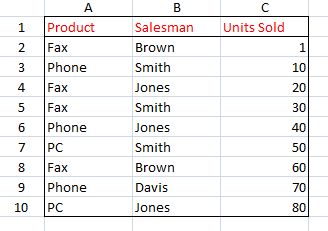
Consider the table of data shown to the right. It lists the number of
products (column C) in different categories (column A) sold by various
salesman (column B). To calculate the number of Fax machines sold
by Brown, we can use the following array formula:
=SUM((A2:A10="Fax")*(B2:B10="Brown")*(C2:C10))
This function builds three arrays. The first array is a series of
TRUE or FALSE
values which are the results of comparing A2:A10 to the word "Fax".
(Remember, Excel will expand the single "Fax" element to an array of
items all of which are "Fax".) The second array is also a series of
TRUE or FALSE
values, the result of comparing B2:B10 to "Brown". (The single
"Brown" element in the formula is expanded to an array of the
appropriate size.) The third array is
comprised of the number of units sold from the range C2:C10. These three
arrays are multiplied together. When you multiply two arrays, the result
is itself an array, each element of which is the product of the
corresponding elements of the two arrays being multiplied. For example,
{1, 2, 3} times {4,
5, 6} is {1*4, 2*5, 3*6} = {4, 10, 18}.
When TRUE and FALSE
values are used in any arithmetic operation, they are given the values 1
and 0, respectively. Thus in the formula above, Excel expands the
formula into the three arrays:
(A2:A10="Fax")� {TRUE, FALSE, TRUE, TRUE, FALSE,
FALSE, TRUE, FALSE, FALSE}
(B2:B10="Brown")� {TRUE, FALSE, FALSE, FALSE,
FALSE, FALSE, TRUE, FALSE, FALSE}
(C2:C10) � {1, 10, 20, 30, 40, 50, 60, 70, 80}
When these array are multiplied, treating TRUE
equal to 1 and FALSE equal to 0, we get the
array
{1, 0, 0, 0, 0, 0, 60, 0, 0}
which are the quantities of Brown's two Fax sales. The
SUM function simply adds up the elements of
the array and return a result of 61, the number of Fax machines sold by
Brown.
You may have noticed that the logic of the formula tests Product equals "Fax" AND Salesman
equals "Brown", but nowhere do we use the AND
function. Here, we use multiplication to act as a logical AND
function. Multiplication follows the same rules as the
AND operator. It
will return TRUE (or 1) only when both of the parameters
are TRUE (or <> 0). If either or both parameters are FALSE (or 0), the
result is FALSE (or 0).
In addition to the logical AND operation using multiplication shown
above, other logical operations can be performed arithmetically.
A
logical OR operation can be accomplished with addition. For example,
=SUM(IF(((A2:A10="Fax")+(B2:B10="Jones"))>0,1,0))
will count the number of sales (not the number of units sold) in which
the product was a Fax OR the salesman was Jones (or both). Addition acts as an OR
because the result it TRUE (or <> 0) if either one or both of the
elements are TRUE (<> 0). It is FALSE ( = 0) only when both elements are
FALSE (or 0). This formula adds two arrays: the results of the
comparisons A2:A10 to "Fax", and the results of the comparisons B2:B10
to "Jones". Each of these arrays is an array of TRUE and FALSE values,
each element being the result of comparing one cell to "Fax" or "Jones".
It then adds these two arrays. When you add two arrays, the result is
itself an array, each element of which is the sum of the corresponding
element of the original arrays. For example, {1,
2, 3} + {4, 5, 6} = {1+4, 2+5, 3+6} = {5, 7, 9}. For each element
in the sum array
(A2:A10="Fax")+(B2:B10="Jones"),
if that element is greater than 0, IF returns 1, otherwise it returns 0.
Finally, SUM just adds up the array.
An "exclusive or" or XOR operation is a comparison that returns TRUE
when exactly one of the two elements is TRUE. XOR is FALSE if both
elements are TRUE or if both elements are FALSE. Arithmetically,
we can use the MOD operator to simulate an XOR operation. For example,
to count the number of sales in which the product was a Fax XOR the
salesman was Jones (excluding Faxes sold by Jones), we can use the
following formula:
=SUM(IF(MOD((A2:A10="Fax")+(B2:B10="Jones"),2),1,0))
A "negative and" or NAND operation is a comparison that returns
TRUE when neither or exactly one of the elements is TRUE, but returns FALSE
if both elements are TRUE. For example, we can count the number of sales
except those in which Jones sold a Fax with the formula:
=SUM(IF((A2:A10="Fax")+(B2:B10="Jones")<>2,1,0))
When you are constructing some types of array formulas, you need to create a
sequence of numbers for a function to process as an array. As an example,
consider an array formula that will compute the average of the Nth largest
elements in a range. To do this, we will use the LARGE
function to get the largest numbers, and then pass those numbers as an array to
AVERAGE to compute the average. Normally, the
LARGE function takes as parameters a range to
process and a number indicating which largest value to return (1 = largest, 2 =
second largest, etc.,). But LARGE does work with
arrays for its second parameter. You might be tempted to type in the array in
the formula yourself: =LARGE(A1:A10,{1,2,3}).
While this will indeed work, it is tedious.
Instead, you can use the ROW function to return a
sequence of numbers. When used in an array formula, the function
ROW(m:n) will return an array of integers from
m to n. Therefore, we
can use ROW to create the array to pass to
LARGE. This changes our array formula to
=LARGE(A1:A10,ROW(1:3)). This brings us
closer to a good formula, but two things remain.
First, if you insert a row
between rows 1 through 3, Excel will change the row reference
1:3, and therefore the formula will average the
wrong numbers. Second, the formula is locked into the three largest values. We can make
it more flexible by making the number of elements to average a cell reference
that can be easily changed.
For example, we can specify that cell C1 contains the size of the array to pass
to LARGE. This is accomplished with the INDIRECT
function. (Click here for more information about
INDIRECT.) The INDIRECT
function converts a string representing a cell reference into an actual cell
reference. The sub-formula ROW(INDIRECT("1:"&C1))
will return an array of numbers between 1 and the value in cell
C1. Now, coming together the formula to average the
N largest values in A1:A10 becomes:
=AVERAGE(LARGE(A1:A10,ROW(INDIRECT("1:"&C1))))
The other type of array formula is one that returns an array of numbers as its
result. These sort of array formulas are entered into multiple cells that are
then treated as a group. For example, consider the formula
=ROW(A1:A10). If this is entered into one cell, either as a normal
formula or as an array formula, the result will be 1 in that single cell. If,
however, you array enter it into a range of cells each cell will contain one
element of the array. To do this, you first must select the range of cells in to
which the array should be written, say C1:C10, type the formula
=ROW(A1:A10), and then press
CTRL SHIFT ENTER. The
elements of the array {1, 2, ...., 10} will be
written to the range of cells, with one element of the array in each cell. When
you array enter a formula into an array of cells, Excel prevents you from
modifying a single cell with that array range. You may select the entire range,
edit the formula, and array-enter it again with CTRL SHIFT ENTER, but you cannot
change a single element of the array.
Some of the built-in Excel functions return an array of values. These formulas must be entered into an array of cells.
For example, the MINVERSE function returns the inverse of a matrix with an equal number of
rows and columns. Since the inverse of a matrix is itself a matrix, the MINVERSE function
must be entered into a range of cells with the same number of rows and columns as the matrix to be inverted. Therefore,
if your matrix is in cells A1:B2 (two rows and two columns), you must select a
range the same size, type the formula =MINVERSE(A1:B2) and press
CTRL SHIFT ENTER rather than just ENTER. This enters the formula as
an array formula into all the selected cells. If you were to use the MINVERSE function in
a single cell, only the upper left corner value of the inverted matrix would be returned.
For information about writing your own VBA functions that return arrays, see Writing Your
Own Functions In VBA.
Array formulas can do a wide variety of tasks. A few miscellaneous array formulas are shown below:
Sum Ignoring Errors
Normally, if there is an error in a cell, the SUM function will return that error. The following
formula will ignore the error values.
=SUM(IF(ISERROR(A1:A10),0,A1:A10))
Average Ignoring Errors
This formula will ignore errors when averaging range.
=AVERAGE(IF(ISERROR(A1:A10),FALSE,IF(A1:A10="",FALSE,A1:A10)))
Average Ignoring Zeros
This formula will ignore zero values in an AVERAGE function.
=AVERAGE(IF(A1:A10<>0,A1:A10,FALSE))
Sum Of Absolute Values
You can sum a range of number treating them all as positive using the ABS function.
=SUM(ABS(A1:A10))
Sum Of Integer Portion Only
This formula will sum only the integer portion of the numbers in A1:A10. The fractional portion
is discarded.
=SUM(TRUNC(A1:A5))
Longest Text In Cells
This formula will return the contents of the cell with the longest amount of text in it.
=OFFSET(A1,MATCH(MAX(LEN(A1:A10)),LEN(A1:A10),0)-1,0,1,1)
There is considerable overlap between what you can accomplish with array formulas and what you can do with the so called
D-Functions (DSUM, DCOUNT, and so on). Broadly speaking, the
D-Functions are faster than their array formula counterparts. If you have a large and complex workbook with many array
formulas, you may see a significant improvement in calculation time if you convert your array formulas to D-Functions.
The primary differences between the D-Functions and array formulas are as follows:
- D-Functions are typically faster than array formulas, all else being equal
- The selection criteria in a D-Function must reside in cells. Array formulas can include the selection criteria directly in the formula
- D-Functions can return only a single value to a single cell, while array formulas can return arrays to many cells
Array formulas are a very powerful tool in Excel, allowing you to do things that
are not possible with regular formulas. Although they may seem complicated at
first, you'll find that with a little practice they are quite logical.
You can download a workbook with the data
and formulas described on this page here.
This page last updated: 7-October-2007