 Eliminating Blank Cells In A Range
This page describes formulas and VBA functions to remove blank cells from a range.

It is not uncommon that you have a range of data containing both values and blank cells and you want to eliminate the blank cells. This page
describes worksheet array formulas and VBA code to create a new range that contains only the non-blank elements
of the original range.
Due to the way array formulas work, it is necessary that the original range
and the new range be referenced by a defined name rather than directly by cell references.
We will use BlanksRange to refer to the original range that contains both values
and blanks, and we will use NoBlanksRange to reference the new range that contains
only the non-blank values of the original range.
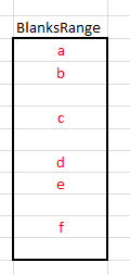
 The image to the left illustrates a
range named BlanksRange that contains a combination of values and blank cells. Although
the values are in alphabetical order, this is by no means necessary. It is for illustration only. The values will be
extracted and will appear in the no-blanks range in the order in which the appear in the original data.
To use the formula, paste it into the first cell of NoBlanksRange and then copy it down
to fill that range. The NoBlanksRange should have as many rows as BlanksRange.
Any unused cells in BlanksRange will contain empty values.
This is an array formula, so you must press CTRL SHIFT ENTER
rather than just ENTER when you first enter the formula and whenever you edit it later, but you do
not array enter it into the entire range at once. Array enter the formula into the first cell of NoBlanksRange
and then fill down to the last cell of NoBlanksRange. The formula is:
=IF(ROW()-ROW(NoBlanksRange)+1>ROWS(BlanksRange)-
COUNTBLANK(BlanksRange),"",INDIRECT(ADDRESS(SMALL(
(IF(BlanksRange<>"",ROW(BlanksRange),ROW()+ROWS(BlanksRange))),
ROW()-ROW(NoBlanksRange)+1),COLUMN(BlanksRange),4)))
The formula above is split into several lines for readability. In practice, it should be entered as a single line. A simpler method is
available in Excel 2007 and later versions, using the IFERROR function.
=IFERROR(INDEX(BlanksRange,SMALL((IF(LEN(BlanksRange),ROW(INDIRECT("1:"&ROWS(BlanksRange))))),ROW(A1)),1),"")
Enter this formula into the first cell of NoBlanksRange and copy it down through the last cell of NoBlanksRange. Like the
other formulas, this is an array formula, so enter it with CTRL SHIFT ENTER rather than just
ENTER. This formula is for extracting the non-blank elements to a vertical range -- a range in a single column that spans several rows.
If you want the results in a single row spanning several columns, use the following array formula, where the result range is named NoBlanksRow.
=IF(COLUMN()-COLUMN(NoBlanksRow)+1>ROWS(BlanksRange)-
COUNTBLANK(BlanksRange),"",INDIRECT(ADDRESS(SMALL(
(IF(BlanksRange<>"",ROW(BlanksRange),COLUMN()+ROWS(BlanksRange))),
COLUMN()-COLUMN(NoBlanksRow)+1),COLUMN(BlanksRange),4)))
Array enter this formula into the first cell of NoBlanksRow and fill to the right through the last cell of
NoBlanksRow.
If the formulas above seem overly complex, you might want to opt for a much simpler VBA function. The NoBlanks function
is shown below.
Function NoBlanks(RR As Range) As Variant
    Dim Arr() As Variant
    Dim R As Range
    Dim N As Long
    Dim L As Long
    If RR.Rows.Count > 1 And RR.Columns.Count > 1 Then
        NoBlanks = CVErr(xlErrRef)
        Exit Function
    End If

    If Application.Caller.Cells.Count > RR.Cells.Count Then
        N = Application.Caller.Cells.Count
    Else
        N = RR.Cells.Count
    End If

    ReDim Arr(1 To N)
    N = 0
    For Each R In RR.Cells
        If Len(R.Value) > 0 Then
            N = N + 1
            Arr(N) = R.Value
        End If
    Next R
    For L = N + 1 To UBound(Arr)
        Arr(L) = vbNullString
    Next L
    ReDim Preserve Arr(1 To L)
    If Application.Caller.Rows.Count > 1 Then
        NoBlanks = Application.Transpose(Arr)
    Else
        NoBlanks = Arr
    End If
End Function
�
This code does not require the use of any defined names. Simply array enter the formula NoBlanks into the entire range
that is to get the results, passing to the function the range from which the blank elements are to be extracted. To array enter the formula into all
the cells, first select the entire range that is to receive the results, enter =NoBlanks(A1:A10) in the first cell and
press CTRL SHIFT ENTER.
The code is written to be entered into a single column spanning several rows or a single row spanning several columns. If the number of rows and the number of columns
of the input range are both greater than 1, the function will return a #REF error. The function will orient itself so that there is no
difference between entering it into a row or into a column. Moreover, if the function is called from a range with more elements than there are non-blank elements,
the results at the end of the result list will filled out with empty string to the full length of cells into which it was entered.
-->

 |
This page last updated: 5-February-2011. |