Matrix To Vector

This page describes Excel worksheet formulas for extracting a vector from a matrix.
ShortFadeBar

There may be circumstances in which you need to extract a vector from a matrix or to convert a matrix to a vector. For our purposes here, we will define a Matrix to be a two dimensional array with at least two rows and at least two columns. We will define a Vector to be a one dimensional array that is either 1 row or 1 column of the Matrix. As an example, we will use the following matrix in the range C10:F12:

Matrix1

This matrix is made up of three row vectors each with four elements and four column vectors each with three elements. The entire matrix has the defined name Matrix.

The first formula we will look at converts the entire matrix to a single column. The order of elements in the resulting column is by row. The values are taken from each row, moving across then down. Enter the following formula into cell C13 and then fill down for 12 rows, or as many cells as are in Matrix.

=OFFSET(Matrix,TRUNC((ROW()-ROW($C$13))/COLUMNS(Matrix)),MOD(ROW()-ROW($C$13),COLUMNS(Matrix)),1,1)

This will transform the array Matrix to a single column of values. Change the reference to cell $C$13 to the first cell in which you entered the formula.

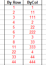
The next formula is similar to the formula above, except that the elements of Matrix are returned column by column, moving down one column and then across to the right to the next column. Enter the following formula in cell D13 and fill down for 12 rows, or as many cells as are in Matrix.

=OFFSET(Matrix,MOD(ROW()-ROW($D$13),ROWS(Matrix)),TRUNC((ROW()-ROW($D$13))/ROWS(Matrix)),1,1)

An abbreviated sample of the column vectors returned from Matrix is shown below:

ColumnVector

You can also use a formula to convert the Matrix to a Row vector. The following formula will transform Matrix into a single row, moving by rows -- left to right on one row and then moving down to the next row. Enter this formula into cell G16 and fill across to the right 12 columns, or as many columns as there are cells in Matrix.

=OFFSET(Matrix,TRUNC((COLUMN()-COLUMN($G$16))/COLUMNS(Matrix)),MOD((COLUMN()-COLUMN($G$16)),COLUMNS(Matrix)),1,1)
Change the reference to $G$16 to the first cell in which you enter the formula.

A similar formula can be used to transform Matrix into a row, ordered by columns. The order of the elements is down one column and then moving to the right to the next column. Enter the following formula in cell G17 and fill to the right for as many columns as there are cells in Matrix.

=OFFSET(Matrix,MOD((COLUMN()-COLUMN($G$17)),ROWS(Matrix)),TRUNC((COLUMN()-COLUMN($G$17))/(ROWS(Matrix))),1,1)

An abbreviated image of the row vectors from Matrix is shown below:

RowVector

You can use a formula to return one row from the Matrix. Name a cell WhatRow and array-enter the following formula into as many columns as there are in Matrix. Note that since this is an array formula that returns an array of values, you must select the cells in which the results are to be returned, type the formula, and then press CTRL SHIFT ENTER rather than just ENTER. If you do this properly, Excel will display the formula in the Formula Bar enclosed in curly braces { }. See the Array Formulas Page for more information about array formulas.

=OFFSET(Matrix,WhatRow-1,0,1,COLUMNS(Matrix))

Change the value of the WhatRow cell to indicate which row to return from Matrix. This value should be 1-based: 1 is the first row, 2 is the second row, and so on.

A similar formula can be used to return one column of Matrix. Name a cell WhatColumn, and then array-enter the following formula into a range of cells with as many rows as there are in Matrix.

=OFFSET(Matrix,0,WhatColumn-1,ROWS(Matrix),1)

You can change the value of the cell WhatColumn to return a specified column of Matrix. This is a 1-based value -- 1 is the first (left-most) column, 2 is the second column, and so on.

You can use the vector formulas to create a dynamic chart that updates its values based on a choice of a row in a matrix of raw data. For example, suppose in cells B6:B9 you have persons' names. Assign the name People to this range. Then, in cells C6:H9, enter some numbers. Assign the name AllScores to this range. Then name a cell Person and add a list-type validation to this cell using the range People as the list source. Next, name the range B16:G16 PersonScores, and in that range array-enter the formula:

=OFFSET(AllScores,MATCH(Person,People,0)-1,0,COLUMNS(AllScores))

Finally, create a chart that pulls its data from the range AllScores. Now, as you change the person name in the cell Person, the chart will automatically update the values to that person's score. A complete example of dynamic charting is shown in the downloadable workbook.

For formulas that do the reverse of the formula on this page, specifically change a single row or column to a matrix, see Vector To Matrix page.