 Ranking Data In Lists
This page describes worksheet formulas you can use to work with data ranking in Excel worksheets.

Excel is often used to keep track of data that needs to be ranked. This might be anything from sports scores to
sales data. Excel provides a worksheet function named RANK that you can use to do rudimentary
ranking, but this function is rather limited. However, we can use some worksheet formulas to provide a much deeper and
meaningful anlaysis of data using the RANK function.
You can an example workbook with the formulas described on this page.

The simplest use of ranking is to get the rank of one or more values in a list. The rank of a number in a list is the
position at which the value would be placed if the data list were sorted. The RANK function does
exactly this and it supports ranking unsorted data, assigning ranks in either ascending order or descending order. Descending
order is the default for the RANK function. In descending order, the higher score is
given the numerically lower rank. For example, if you have bowling scores of {150, 125, 180, 175},
the value 180, the highest value in the list, is given a rank of 1 and the value
125, the lowest value in the list, is given the rank of 4. Even though in common language usage, the
highest score is said to be the "highest ranked" score, the actual numeric value of the rank is the lowest. (E.g., "the highest
ranked bowling score was 180", may sound correct, but the rank of 180 is actually the lowest rank value, 1).
When you rank in ascending order, the lower values are given the numerically lower rank. Golf scoring is an
example in which you would use ascending ranking. The lower the score the better, so lower values are assigned lower
numerical rankings. With the scores {72, 88, 75, 82}, the value 72,
the lower score in the list, is given a rank of 1 and 88, the highest score in the list, is given a rank of 4.
The RANK function is essentailly the inverse of the LARGE (and
SMALL) function. While RANK returns the rank of a value in a list,
LARGE returns a value based on its rank. If cells B4:B8 contain
the values {5,2,4,3,1}, the formula =LARGE($B$4:$B$8,RANK(B4,$B$4:$B$8,0)) in
cells C4:C8 returns the original data in the original order, confirming the relationship between
RANK and LARGE. A similar formula can be created with the
SMALL function: =SMALL($B$4:$B$8,RANK(B4,$B$4:$B$8,1)).
One of the features (or failures, depending on your perspective) of the RANK function is that it
returns the same rank value for items of equal value. For example, with the data {33, 22, 44, 22, 11}
the RANK function returns a rank of 1 to the value 44, the value 2 for 33, the value 3 for both
occurrences of 22, and then a rank of 5 for 11. No value is ranked as 4. You can use a formula to prevent this duplication of
rank value. For example, the following formula entered in cell B1 and filled down to
B5 will return unique ranks of the values in A1:A5
=RANK(A1,$A$1:$A$5,0)+COUNTIF($A$1:A1,A1)-1
To see how this formula works, enter the values 33, 22, 44, 22, 11 in cells
A1:A5 and enter the formula =RANK(A1,$A$1:$A$5,0)+COUNTIF($A$1:A1,A1) in
cell B1. Fill the formula down from B1 through
B5. This will return the values 2, 3, 1, 4, 5 to cells
B1:B5. Examine the formulas in cells B2 and B4,
the cells that are adjacent to the duplicated value 22. In B2, the RANK
returns 3 (as it should), and the COUNTIF function is
COUNTIF($A$1:A2,A2) which returns 1. Subtract 1 from the result of COUNTIF and you'll get 0,
which when added to the value 3 from RANK gives us 3, the correct rank of the first occurrence of
22. Now, look at the formula in cell B4, which is adjacent to the second occurrence of the value
22. As before, the RANK function returns 3, but the COUNTIF function is
now COUNTIF($A$1:A4,A4) which returns 2, the number of values 22 in
range A1:A4. Subtract 1 from that result and add that to the result of RANK,
and you'll get 4. This formula will work with any number of duplicated values. The reason that it works is that for any value
V that occurs N times in a list, with a rank of
R, there are N rank values R, and the next
N-1 occurrences of V have the rank R. This
means that N-1 rank values are omitted and the next rank value is R-N.
The COUNTIF()-1 piece of the formula adds back N-1, and
R+N-1 is the rank of the Nth occurrence of the value
V. For as many occurrences N of V
exist in the list, the RANK function omits N-1 rank value. The
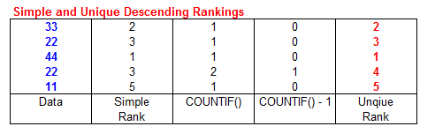
COUNTIF()-1 simply adds those missing rank values back into the ranking. In the following
screen shot, the original data values to be ranked are shown in blue, the intermediate
calculated results in black, and the final results shown in .
The logic for unique ascending ranks is a bit different than that for descending unique ranks. With your data in the range
A1:A5, enter the following formula in cell B1 and fill down to cell
B5.
=COUNT($A$1:$A$5)-(RANK(A1,$A$1:$A$5)+COUNTIF($A$1:A1,A1)-1)+1
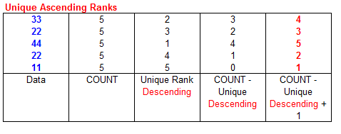
The formula works in the following manner. The total number of elements minus the descending rank of a value is that
value's ascending rank as if the rankings were 0-based rather than 1-based. For example, the unique
descending rank of the value 33 is 2. Subtracting this from the total number of elements, 5, returns the zero
based rank of 3. Adding 1 brings the rank to a 1-based system and therefore 33 gets the rank of 4. It is important to
note that even though this formula calculates the ascending ranks, it uses the descending format of
the RANK function. In the screen show below, the data to be ranked is shown in
blue, the intermediate calculations in black, and the
final results in red.
While the formulas illustrated above are useful for the direct ranking of data, it is very often the case that you want to
return a ranked list of the players or other entities that have ranked scores or values. For example, a ranking of bowling
scores is useful really only when you can retrieve the players in scored rank. The actual scores are less useful than are
the player names themselves. This section will create a list of players according to the ranked scores, in descending rank
order.
In the following example, the player names are in B4:B13 and each player's score is in
C4:C13. We use the following formula to calculate the unique descending rankings of the players'
scores. This is the same formula descibed earlier in this article.
=RANK(C4,$C$4:$C$13,0)+COUNTIF($C$4:C4,C4)-1
Enter this formula in cell E4 and fill down to E13. This gives us
the unique rankings of the player's scores that we will use to retrieve the player names in scored order. Enter the following
formula in cell G4 and fill down to G13. This will list the names of
the players, listed in B4:B13 in the order of the unique ranks
in E4:E13.
=OFFSET(B$4,MATCH(SMALL(E$4:E$13,ROW()-ROW(G$4)+1),E$4:E$13,0)-1,0)
In the screen image below, the input data is shown in blue, the unique rankings in
black, and the final results in .
The previous section display players ordered by a descending unique rank. The same players may be ordered by ascending rank order.
With the player names in cells B18:B27 and their scores in cells C18:C27,
enter the following formula in E18:E27
=COUNT($C$18:$C$27)-(RANK(C18,$C$18:$C$27,0)+COUNTIF($C$18:C18,C18))+2
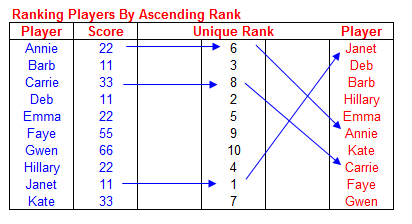
This formula will create unique player ranks in ascending order. These ranks will be used to create the order list of players. In
cell G18, enter the following formula and fill it down to cell G27.
=OFFSET(B$18,MATCH(SMALL(E$18:E$27,ROW()-ROW(G$18)+1),E$18:E$27,0)-1,0)
This will list the players in ascending rank order. The screenshot below illustrates this.
In the examples above, we had tied scores, two players having the same score. In those scenarios, there was no way to break a tie.
The tied elements would appear in the result list according to their position in the input list. This section of the article
describes how to use multiple tables to resolve ties. We first have a primary table that contains the players name
and their scores. Next, we have a secondary table that is used to resolve ties. If two player have the same score
in the primary table, those players' scores in the secondary table are used to break the tie. (If those same player have a tied
score in the secondary table, the results are returned in the order in which they appear in the secondary list.
The core of working with the two lists and breaking the ties in to create a third table, called the Composite table. This
table lists all of the player and calcualtes a composite rank that is calculated from the player's rank in the primary table and
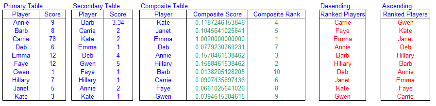
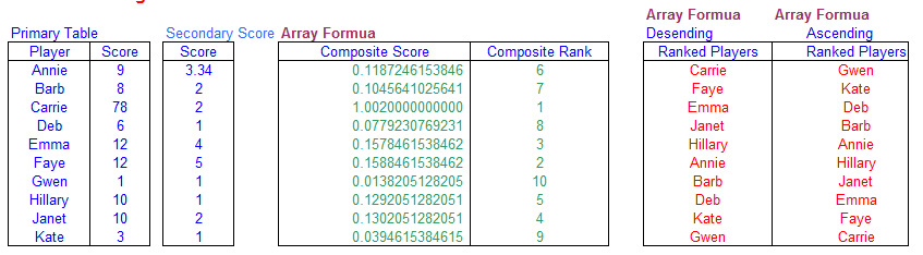
her rank in the secondardy table. Assuming you have the primary table with player names and scores in the range
B6:C15, called Table1, the secondary table, also wih player
names and scores, in cells E6:F7, named Table2,
and the composite table in cell H6:J16, with Player Names in column H,
the composite score (to be calcuated later) on column I, and the Composite Rank (also discussed later)
in column J, you can list the players by score in descending rank in column L
and the players by score in acsendning rank in column N. The basic layout of the tables is
shown below. The rest of this section will discuss how write the formula and what those formulas actually do.
The formulas on this page are Array Formula, so you must press CTRL SHIFT ENTER rather than ENTER when you first enter the
formula and whenever you edit it later. If you do this correctly, Excel will display the formulas enclosed in curly braces
{ }. See the Array Formulas page for more information about
working with array formulas.
In the cells of column I in Table1 enter the following formula:
=(C6/MAX(ABS($C$6:$C$15)))+(F6/(10^(MAX(LEN(C$6:C$15)+1))))
This formula calculates the Composite Score. This score is calculated with the following formula:
=(C6/MAX(ABS($C$6:$C$15)))+(F6/(10^(MAX(LEN(C$6:C$15)+1))))
For each row in the Composite Score, this calcualtes the data value divided the maximum data element. This number,
N is subject to constraint 0 <= N <= 1. Added to this is is the value
of the secondary (tie breaking) rank divided by (10^(MAX(LEN($C$6:$C$15)+1). This calculated value
is 10 to power of Z where Z is the longtest (in terms of character length,
not numeric value) of the numbers in cells C6:C15. If the longest number has six characters (e.g.,
123.456), the formula (10^(MAX(LEN($C$6:$C$15)+1) reutrns 10^7. When we divide that into the cell
value from the score from the secondary table, we get a fractional number that is 0's until the number of digits surpass the
digit to right of the decimal point from the score value from Table2. Finally, to break ties between scores in Table2, we
divide the current Row number by ((ROW()/(10^MAX(LEN($F$6:$F$15)+1)))). This ensure that the least significant
protion of the number is scaled past the end of the decimal number to which it is added.
One we have composite score, which combines the scores in the primary and second tables to generate a unique, properly ordered key,
we must rank the composite scores. We do this with the same formula we used earlier in this to determine unique ranks. In cell
J6, enter the following formula and then fill down to J15.
=RANK(I6,$I$6:$I$15,0)+COUNTIF($I$6:I6,I6)-1
This is just the unique rank of the composite scores. Finally, after all this, we can use the composite ranks to return the names
of the players in either Descending or Ascending order. To return the list in Descending order, enter the formula in
cell L6 and fill down to L15.
=OFFSET(B$6,MATCH(SMALL(J$6:J$15,ROW()-ROW(J$6)+1),J$6:J$15,0)-1,0)
To return the names in Ascending order, enter the following formula in cell N6 and fill down to
N15,
=OFFSET(B$6,MATCH(LARGE(J$6:J$15,ROW()-ROW(N$6)+1),J$6:J$15,0)-1,0)
As a practical matter, you don't need to include the player names in any table other than the primary tab. As longs as everything
is in the same rows, you can simply the display to the following:
You can an example workbook with the formulas described on this page.
This page last updated: 19-Sept-2007