 Duplicate Data In Lists
This page describes techniques for dealing with duplicate items in a list of data.

Very often, Excel is used to manage lists of data, such as employee names or phone
lists. In such circumstances, duplicates may exist in the list and need to be identified.
This page contains a number of formulas that can be used to work with duplicate
items in a list of data. All the formulas on this page are array formulas.
DEFINITION: Array Formula
An array formula is a formula that works with arrays or series of data rather than single data values. When you
enter an array formula, type the formula in the cell and then press CTRL SHIFT ENTER
rather than just ENTER when you first enter the formula and when you edit it later.
If you do this properly, Excel will display the formula enclosed in curly braces { }. Array
formulas are discussed in detail on the Array Formulas page.
You can download an example workbook here that illustrates all the
formulas on this page.
For a VBA Function that returns an array of the distinct items in a range or array, see the Distinct
Values Page. This function can be called either from a range of worksheet cells or from other VB code.

The formula below will display the words "Duplicates" or "No Duplicates" indicating
whether there are duplicates elements in the list A2:A11.
=IF(MAX(COUNTIF(A2:A11,A2:A11))>1,"Duplicates","No Duplicates")
An alternative formula, one that will work with blank cells in the range, is shown
below. Note that the entire formula should be entered in Excel on one line.
=IF(MAX(COUNTIF(INDIRECT("A2:A"&(MAX((A2:A11<>"")*ROW(A2:A11)))),
INDIRECT("A2:A"&(MAX((A2:A11<>"")*ROW(A2:A11))))))>1,"Duplicates","No
Duplicates")
You can use Excel's Conditional Formatting tool to highlight duplicate entries in
a list. All of the examples in this section assume that the data to be tested
and highlighted is in the range B2:B11. You should change the cell references to
the appropriate values on your worksheet.
This first example will highlight duplicate rows in the range B2:B11. Select the
cells that you wish to test and format, B2:B11 in this example. Then, open the Conditional Formatting dialog from the Format menu, change Cell
Value Is to Formula Is, enter the formula below, and choose a font or background
format to apply to cells that are duplicates.
=COUNTIF($B$2:$B$11,B2)>1
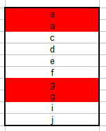
The formula above, when used in Conditional Formatting, will highlight all duplicates. That is, if the value 'abc' occurs twice in the list, both instances of 'abc' will
be highlighted. This is shown in the image to the left, in which all
occurrences of 'a' and 'g' are higlighted.
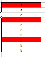
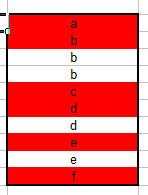
You can use the following formula in Conditional Formatting to highlight only the first occurrence
of an entry in the list. For example, the first
occurrence of 'abc' will be highlighted, but the second and subsequent occurrences
of 'abc' will not be highlighted.
=IF(COUNTIF($B$2:$B$11,B2)=1,FALSE,COUNTIF($B$2:B2,B2)=1)
This is shown
at the left where only the first occurrences of the duplicate items 'a',
'e', and 'g' are highlighted. The second and subsequent occurrences of these
values are not highlighted.
You can also do the reverse of this with Conditional Formatting. Using the formula
below in Conditional Formatting will highlight only the second and subsequent occurrences
of a value. The first occurrence of the value will not be highlighted.
=IF(COUNTIF($B$2:$B$11,B2)=1,FALSE,NOT(COUNTIF($B$2:B2,B2)=1))
This is shown at the left where only the second occurrences of 'a', 'b',
'c' and 'f' are highlighted. The first occurrences of these items are
not highlighted.
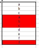
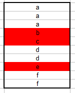
 Another formula for Conditional Formatting will highlight only the last
occurrence of a duplicate element in a list (or the element itself if it
occurs only once).
Another formula for Conditional Formatting will highlight only the last
occurrence of a duplicate element in a list (or the element itself if it
occurs only once).
=IF(COUNTIF($B$2:$B$11,B2)=1,TRUE,COUNTIF($B$2:B2,B2)=COUNTIF($B$2:$B$11,B2))
As you can see only the last occurrences of elements 'a', 'b', 'c', and
'f' are highlighted. Element 'd' is highlighted because it occurs only
once. The occurrences of 'a', 'b', 'c' and 'f' that occurs before the
last occurrence are not highlighted.
We can round out our discussion of highlighting duplicate rows with two additional
formula related to distinct items in a list.
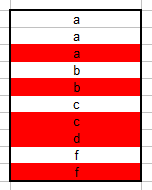
The following can be used in Conditional Formatting to highlight elements
that occur only once in the range B2:B11.
=COUNTIF($B$2:$B$11,B2)=1
This image illustrates the formula. Elements 'b', 'c', and 'e' are
highlighted because they occur only once in the list. Items 'a', 'd' and 'f'
are not highlighted because they occur more than one time in the list.
Finally, the following formula can be used in Conditional Formatting to highlight the distinct
values in B2:B11. If an element occurs once, it is highlighted. If it occurs more
then once, then only the first occurrence is highlighted.
=COUNTIF($B$2:B2,B2)=1
As you can see, only the first or only occurrences of the elements are
highlighted. If an element is duplicated, as is 'b', the duplicate
elements are not highlighted.
All of the formulas described above for Conditional Formatting can also be used
in worksheet cells. They are all array formulas, so you must select the range for
the results, type in the formula, and press CTRL SHIFT ENTER.
The results of each formula will be a series of True or False values. The
True results correspond to those cells that are highlighted in Conditional Formatting
and the False results correspond to those cells that are not highlighted by Conditional
Formatting.
The following formulas will return the number of distinct items in the range B2:B11. Remember, all of these are
array formulas.
The following formula is the longest but most flexible. It will properly
count a list that contains a mix of numbers, text strings, and blank
cells.
=SUM(IF(FREQUENCY(IF(LEN(B2:B11)>0,MATCH(B2:B11,B2:B11,0),""), IF(LEN(B2:B11)>0,MATCH(B2:B11,B2:B11,0),""))>0,1))
If your data does not have any blank entries, you can use the simpler formula below.
=SUM(1/COUNTIF(B2:B11,B2:B11))
If your data does have embedded blank cells within the full range, you can use the following array formula:
=SUM(1/IF(B2:B11="",1,(COUNTIF(B2:B11,B2:B11))))-COUNTBLANK(B2:$B11)
If your data has only numeric values or blank cells (no string text entries), you can use the following formula:
=SUM(N(FREQUENCY(B2:B11,B2:B11)>0))
Additional Information can be found on the following pages:
See Distinct Element In A List
This page last updated:
13-July-2007