Color Banding Based On Content

This page describes how to color groups of rows based on their content.

Introduction

Elsewhere on this site, we looked at a method of using Conditional Formatting (CF) to color groups of rows, creating the look and feel of an accounting ledger page or old fashioned "green bar" computer paper. Those formulas created bands of colors that spanned a specific and unchanging number of rows, regardless of the content of the cells. This page describes how to use CF to band rows based on content. This image illustrates content-based formatting: 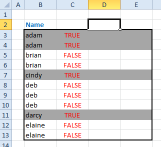In this example, the color banding is based on where the Name value (in column B) changes value. Both of Adam's rows are formatted, but when the value in column B changes from Adam to Brian, the banding stops, and remains off until the name changes again. This pattern will work with groups of any number of rows.

In this description, we'll call the column of data containing the data to be tested the data column. Insert a new column on the worksheet. It doesn't really matter where this column in placed. This will hold the formulas used as the criteria for CF banding; we will refer to that column as the format column. We will assume for purposes of example that the data column begins in B1 and the format column begins in C1. In C1 enter the value TRUE. In C2 enter the following formula:

=IF(B1=B2,C1,NOT(C1))

Copy this formula down the format column (C) for as many rows as there is data in the data column (B) . The banding pattern is what we will call odd banding, meaning that the odd groups of names (first, third, fifth, etc.) will be formatted and the even groups of names (second, fourth, sixth, etc.) will not be formatted. To reverse this, so that the even groups are formatted, change the value in C1 from TRUE to FALSE.

Now, select all the cells to which the conditional formatting will be applied. Typically, this will be the data column and some number of columns to the right. Open the Conditional Formatting dialog and change Cell Value Is to Formula Is (Excel 2003 and earlier) or choose the Use a formula... option (Excel 2007 and later). In the formula box in that dialog, enter =$C1 where C is the format column and 1 is the first row of data. You need to use the $ character as shown in the formula. Click the Format button and choose the format that is to be applied to the cells.

Now that you've finished applying the Conditional Formatting, you should see results similar to the image above. You can hide the format column to make your worksheet look cleaner. The formulas will continue to work just fine with the column hidden.

You can download the file with all the example formulas on this page.

This page last updated: 10-December-2010.