Color Banding With Conditional Formatting
In Excel97 and later versions, you can
use the Conditional Formatting tool to create color bands in your rows, so
that it appears as accounting ledger sheets or computer "green
bar" paper. The advantage of using Conditional Formatting to
change the colors, rather than manually shading the cells, is that the
colors will not get moved when you sort the worksheet or when you insert
or delete rows or when you sort rows. For
more information about Conditional Formatting, click
here.
|
|||
Odd And Even Banding
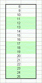
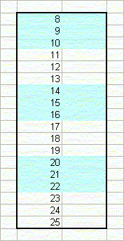
The left image shows what is called "odd banding". This means that the odd bands are colored and the even bands are left plain. Here, bands 1, 3, and 5 are colored in light blue, and the even bands, 2, 4, and 6 are left plain. Similarly, the right image shows what is called "even banding". This means that the even bands, 2, 4, and 6 are colored, while the odd bands, 1, 3, and 5, are left plain. Note that "odd" and "even" refer to the groups of rows, not the number of rows in each band, and not the the row numbers.
|
|
||
Formulas For Color Banding
The formulas for odd banding and even banding are very similar. For odd banding, use the formula =MOD(ROW()-Rw,N*2)+1<=N where Rw is the first row number that is to be formatted, and N is the number of rows in each color band. In the example shown on the left above, Rw is 8, and N is 3. For even banding, use the formula =MOD(ROW()-Rw,N*2)+1>N where Rw is the first row number that is to be formatted, and N is the number of rows in each color band. In the example shown on the right above, Rw is 8, and N is 3.
|
|
||
To use these formulas in Conditional Formatting, select
the cells that you want to format. Then, go to the Format menu, and
choose Conditional Formatting. In this dialog, change "Cell Value
Is" to "Formula Is", and enter one of the formulas
above.
|
|
In both formulas, you can either put it
literal values for Rw and N, or you can create defined names and store the
value there. An advantage to using defined names is that you can
change to band height very easily. To shade alternate rows,
simply change N to 1. To shade in bands of 5, change N to
5. If you are storing the values of N and Rw in other worksheet
cells, as is done in the example workbook,
be SURE to use absolute, not relative, cell
referencing to reference these values.
And because the Conditional Formatting formulas are not moved with the cells when you sort a range, the bands will remain intact after the sort. |